Explanation of the Mathematics

From the previous section we see that there are clearly many ways to approximate pi. However, it is also important to understand the "how" and "why" behind each of these approximation methods. Here, we will look at the mathematics behind just a few of these approximations. The first historically significant method of approximating pi was using Archimedes' method. Beginning with a circle with a radius of length 1, one can inscribe and circumscribe a regular n-gon about the circle. The inscribed n-gon will have a perimeter which is smaller than the circumference of the circle, while the circumscribed n-gon will have a perimeter which is larger than the circumference of the circle. As the number of sides of each polygon is increased, each polygon resembles the circle more and more, and thus their perimeters become increasingly closer to the measure of the circumference of the circle.

Image courtesy of Better Explained

Recalling that we understand the equation of the circumference of a circle to be \(C=2\pi r\), this means that as we increase the number of sides on our polygons, the perimeters of those polygons will get closer and closer to the value of \(2\pi r\). If the length our radius is indeed 1, as we have assumed, then really each polygon perimeter is approaching the value \(2\pi\). Thus, dividing the perimeter of either of the polygons by 2 gives an approximation of pi, with the inscribed polygon giving a slightly low estimate for pi and the circumscribed polygon giving a slightly high estimation for pi. These values represent upper and lower bounds for the value of pi. Essentially, pi is trapped between them. Furthermore, recalling that Archimedes also proved the area of a circle to be \(A=\pi r^2\), the area of a circle with radius 1 is in fact \(\pi\). Since the areas of our polygons also approach the area of the circle as more sides are added, the areas of our polygons can be used as estimations of pi in a similar fashion to their perimeters, meaning as upper and lower bounds. The perimeter method is essentially the one Archimedes used to approximate pi. He began with a hexagon, then doubled the number of sides until he was working with a 96-sided polygon and calculated that \(3\frac{10}{71} < \pi < 3\frac{10}{70}\) (Borwein & Chapman, 2015).

Another method of estimating pi, which also uses some geometric aspects, is something called the Monte Carlo Method. Consider a square circumscribed about a circle. Now suppose you were to somehow randomly generate dots within the square. Some of those dots would fall within the square and the circle, while others would only fall within the boundaries of the square (Estimating Pi Using the Monte Carlo Method, 2017). Note that we know that the area of the circle must be \(A=\pi r^2\) and the area of the square is \(A=4r^2\). If we divide the area of the circle by the area of the square, we would get \(\pi/4\), and this same ratio "can be used between the number of points within the square and the number of points within the circle. Hence we can use the following formula to estimate pi: \(\pi = 4 * (\text{the number of points in the circle}/\text{the number of total points})\)" (Estimating Pi Using the Monte Carlo Method, 2017). This approximation increases in accuracy the more random points are generated.

Applet by Jon McLoone found on Wolfram

Yet another interesting and innovative way to approximate pi is through the use of a problem from the field of geometrical probability which was first stated in 1777 (Safronov, 2005). This problem involves dropping a needle onto a lined piece of paper where the lines are equally spaced. Determining the probability of the needle crossing one of the lines on the page is actually directly related to the value of pi (Safronov, 2005). To explain why, we'll look at the simplest case where the needle is of length 1 and the lines are spaced one unit apart. When dropping a needle, there are two variables to take into consideration: 1) the angle at which the needle falls which we'll refer to as \(\theta\) and 2) the distance from the center of the needle to the closest line which we'll refer to as D. "Theta can vary from 0 to 180 degrees and is measured against a line parallel to the lines on the paper. The distance from the center to the closest line can never be more than half the distance between the lines"(Safronov, 2005). It was discovered that the needle will hit the line if \(D \leq \frac{1}{2} \sin(\theta)\), but how often does this occur? Consider the graph below:

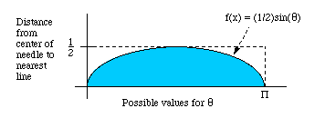
In this graphical representation of the problem, any value that falls on or below the curve represents when the needle will cross the line (Safronov, 2005). That is, the shaded region represents when \(D \leq \frac{1}{2} \sin(\theta)\). Note that the area of the shaded portion is equal to \( \int_{0}^{\pi} \frac{1}{2} \sin(\theta) \, d\theta = 1 \) and the area of the entire rectangular area is \(\frac{\pi}{2}\) (Safronov, 2005). So the probability of a line-cross is \(\frac{1}{\pi/2}=\frac{2}{\pi}\). Note that we can represent this more generally in the following way: \(\frac{\text{hits}}{\text{drops}}=\frac{2}{\pi}\) . What this helps us to see is that if we want to calculate pi from our needle drops, "simply take the number of drops and multiply it by two, then divide by the number of hits... \(2 \times \frac{\text{total drops}}{\text{number of hits}} = \pi\) (approximately)" (Safronov, 2005).

While there are so many wonderful geometric ways to estimate pi, if history tells us anything it's that there are even faster ways using algebraic methods. That is, as discussed earlier, through the use of infinite series. Specifically, we will look at the Gregory-Leibniz formula, which states that \(\frac{\pi}{4}=1-\frac{1}{3}+\frac{1}{5}-\frac{1}{7}+\frac{1}{9}- ...\) (Borwein & Chapman, 2015). Why is this so? Where did it come from? To figure out the logic behind this, let's first look at a familiar geometric series: \(\frac{1}{1-x}=1+x+x^2+x^3+x^4+...\) where \( |x| < 1 \) (MrYouMath, 2014). Now let's plug in \(-x^2\) for \(x\). This gives us \(\frac{1}{1-(-x^2)}=1+(-x^2)+(-x^2)^2+(-x^2)^3+(-x^2)^4+...\) (MrYouMath, 2014). If one was to simplify this, you'd simply get the following: \(\frac{1}{1+x^2}=1-x^2+x^4-x^6+x^8-....\) Now, suppose we found the integral of each side of the equation. \( \int \frac{1}{1 + x^2} \, dx \) is easily recognized as being equal to \(\arctan(x)\) while the integral of the right side is equal to the sum of the integrals of the individual terms. That is, \(\arctan(x)=x-\frac{x^3}{3}+\frac{x^5}{5}-\frac{x^7}{7}+\frac{x^9}{9}-...\) where \( |x| < 1 \) (MrYouMath, 2014). Note that we know \(\tan(\frac{\pi}{4})=1\), which therefore means that \(\arctan(1)=\frac{\pi}{4}\) . Thus, if we were to substitute a 1 into our geometric expansion for the arctangent, we'd get the following: \(\arctan(1)=\frac{\pi}{4}=1-\frac{1}{3}+\frac{1}{5}-\frac{1}{7}+\frac{1}{9}-...\), which is the Gregory-Leibniz formula (MrYouMath, 2014). This further means that one can approximate pi through adding up as many terms in this series as they can, then multiplying this sum by four.

Finally, the last way we will look at the ways in which pi can be approximated is through the use of Riemann sums. Riemann sums are used to approximate the area under a curve. Thus, knowing that a circle with a radius of length one has an area of \(\pi\), if we use Riemann sums to approximate the area of a portion of a unit circle, this can help give us an approximation for \(\pi\). The equation \(y=\sqrt{1-x^2}\) creates a curve, the area under which is one-fourth the area of a unit circle (Theiler, 2021). Using a Riemann sum to calculate the area under this curve, then multiplying it by 4 gives an approximation for \(\pi\) (Theiler, 2021). The more bars used in the Riemann sum, the more accurate the approximation will be.

Applet by Yin Su found on Geogebra