Now that we have finally constructed the major scale, it feels great to know our ratios line up so perfectly. However, they actually do not. If we add up our ratios of 5 whole tones and 2 halftones, we do in fact get a ratio of 2:1, but that is only because a halftone isn’t truly half of a whole tone. A halftone plus another halftone (256:243*256:243) truly equals 65,536:59,049. An easier way to understand this is by comparing 65,536/59,049=1.110 with 9/8=1.125. So, if we define a halftone as exactly half of a whole tone, our scale will be out of tune: slightly sharp. We can see this by showing that the summation of 6 whole tones does not equal an octave (9:8*9:8*9:8*9:8*9:8*9:8=531,441:262,144). This then brings up the question, how does one correctly be in tune? The answer: there is no correct way. There exist many different tuning methods as a result of these fundamental ratios we have explored. In fact, we have already discovered that Pythagorean tuning as strayed from the tuning method suggested by the overtone series. Recalling to the previous overtone image, a major third should be defined as a ratio of 5:4 (or 1.25). However, we discovered that Pythagoras defined a major third as 81:64 (or 1.266). Why do these discrepancies even exist, and what differences do these ratios imply on the overall tuning system? The following video provides great insight into these questions, and helps summarize Pythagoras’ significance on the modern tuning system:
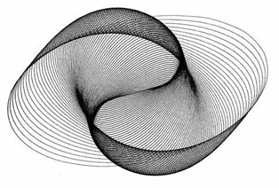
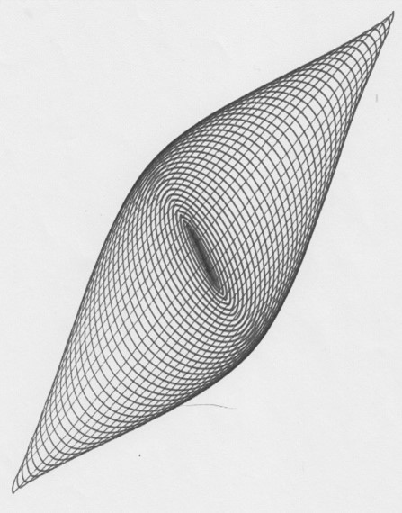
Tuning is only one of many examples of the application of mathematics in music. One geometric application of harmony is something called a harmonograph. The harmonograph is an instrument invented in the mid nineteenth century that draws pictures of musical harmonies (Ashton). The basis of this machine is from an experiment devised by French mathematician Jules Lissajous. In this experiment, Lissajous placed a small mirror on the tip of a tuning fork and aimed a light beam at it. When he did so, he discovered that he could throw the vibration onto a dark screen. Doing this produced a vertical line, but he didn’t stop there. He decided to redirect the beam sideways with another mirror, and this time it produced a sine wave. Now, he decided to replace the mirror with another tuning fork. When he placed this second tuning fork at a right angle to the first, he discovered that tuning forks with relative frequencies in simple ratios (as described by Pythagoras) produced stunning shapes:
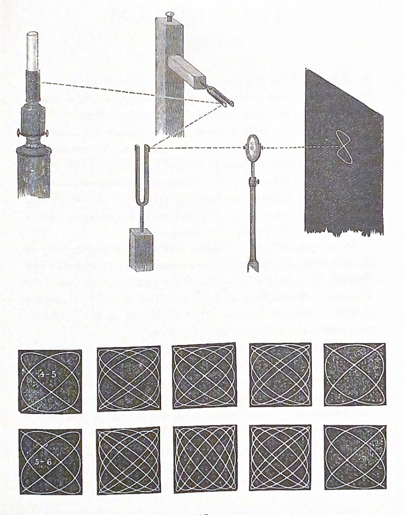
The top image shows that tuning forks an octave apart (2:1) produce a figure eight. In the bottom image, the top row shows a major third (5:4) and the bottom row shows a minor third (6:5) as they phase through different shapes.
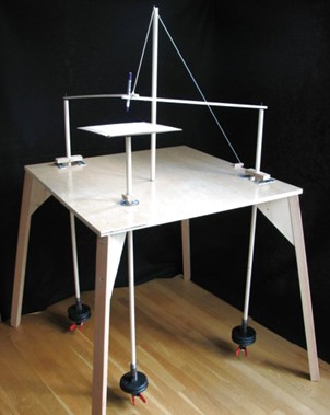
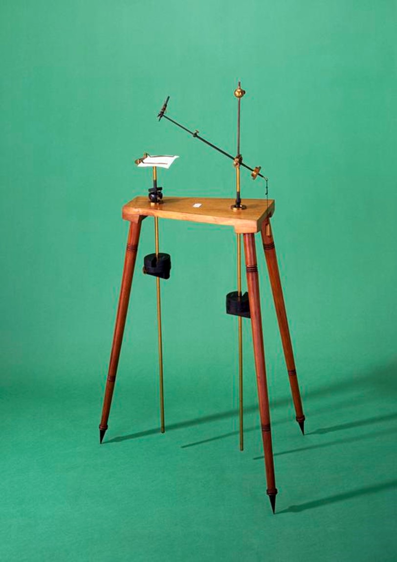
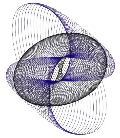
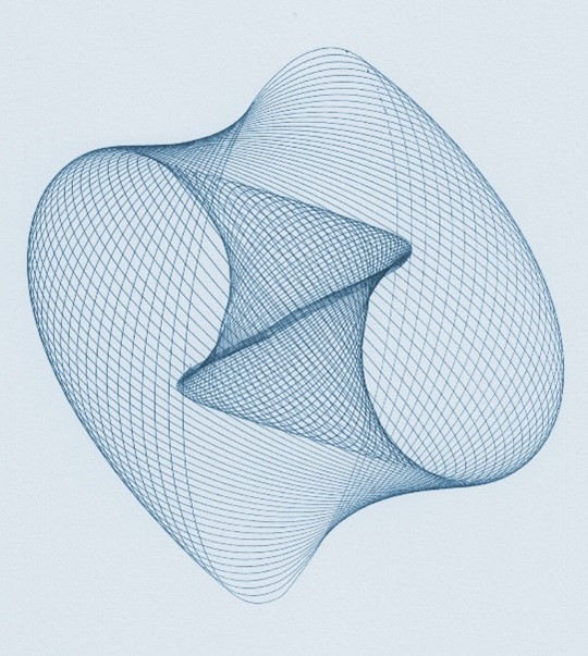
Lissajous experiment paved the way for visualizing harmony, however the harmonograph does not rely on a beam of light to produce harmony. Rather, it relies on two pendula. Galileo discovered that the frequency of a pendulum’s beat is dependent on its length. Because of this, we can use two pendula to represent a harmony: one pendulum with the weight kept at its lowest point, and the other pendulum with the weight moved to wherever will produce the desired ratio. For the simplest harmonograph, the pendula are suspended through holes in a table, swinging with lateral motion perpendicular to one another. With the top of one pendulum carrying an arm with a pen and with the top of the other pendulum sporting a platform with a paper, their combined motion draws an image. The harmonograph can create different images depending on the number of pendula, the type of motion of each pendulum (lateral, rotary, concurrent, countercurrent, etc.), and the desired ratios between them. As we can see, things can get complex quite fast. For the sake of this discussion, this is as far as we will analyze harmonographs, however, it’s intriguing to see what unique applications of harmony can be brought into geometry. Below is an image of two simple harmonographs, as well as images produced from a harmonograph:
One final application of mathematics in harmony is revolved around one person: Jacob Collier. Jacob Collier is a 28-year-old musician from London, England. Despite his young age, he is contributing more to the field of Western music than any other current artist, and his 5 Grammy’s (plus 4 additional nominations) speak to that. What Collier is helping to develop in Western music is microtonality and negative harmony and their implications in not only jazz, but also popular music. The concept of negative harmony is all about polarity and symmetry. Rather than going into an in-depth explanation of what negative harmony is, we will watch Jacob Collier himself explain it (stop at 3:27):
From this video, we can clearly see the mathematical application of negative harmony: we treat notes as points on a plane, establish where our axis is musically, and rotate the notes about the axis in perfect symmetry. However, what do microtones have to do with negative harmony?
Microtones are intervals that are smaller than a halftone. Since Pythagoras’ invention of the twelve-note system became the standard for Western music, microtones don’t exist in Western music. However, as various places in Asia and Africa were developing music independently, they embraced a different system of notes: music that the West would consider microtonal. As Jacob Collier described, if you create an axis between the notes C and G, the axis will be running through a microtone. He lovingly refers to this note as E half-flat. This is because the note exists exactly halfway between E natural and E flat. If we can define the existence of a note exactly halfway between a halftone as we just did, then is it possible to define other notes between halftones? This brings in a concept called cents. A cent is defined as one hundredth of a halftone. With a division on pitch this small, there is no need to divide the halftone any smaller than this, for the human ear can only notice a pitch change of about five cents. With this, we can now define E half-flat instead as being 50 cents sharp of E flat.
Cents have greater implications than just calling notes by different names. By being able to define microtones with numbers rather than with names, we can apply the same proportional ideas that Pythagoras used with his 12-tone system, but with a new twist. If we are thinking in terms of equal temperament, then an octave is comprised of 12 halftones, and with each halftone equaling 100 cents, an octave would equal 1200 cents. Suppose I wanted to play a lick on a magical piano that contained a key for every cent in the octave, with each key being labeled from 0-1200. In this lick, I want to start on C (1200) and end on C an octave lower (0), but I want to get there in 15 equally pitched notes. With this system, we can define what those notes are by dividing 1200 by 15 (1200/15=80) and travelling that many cents each time. In this example, we would be playing the keys labelled 1200, 1120, 1040, 960, 880, 800, 720, 640, 560, 480, 400, 320, 240, 160, 80, finally landing on 0. Now let’s convert these magical keys into real music. If the lower C is defined as 0 and the higher C is defined as 1200, since 100 cents is a halftone, we can create a chart to help us know what Pythagorean halftone our microtones are closest to:
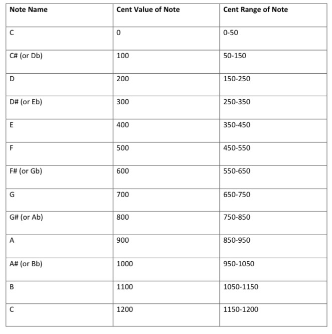
Using this table, we would rewrite our magical piano notes as such: C, B+20cents, Bb+40cents, Bb-40cents, A-20cents, Ab, G+20cents, Gb+40cents, Gb-40cents, F-20cents, E, Eb+20cents, D+40cents, D-40cents, Db-20cents, C. Now that we have married microtonality with Western notation, this unlocks the possibilities of practicing Western music theory on microtonal music.