Significance and Applications
Historical Applications of Logarithms
As discussed in History, logarithms were created to do quick and accurate multiplication. The inception of logarithms led to computational tools, one of the most popular and widely used being the slide rule.In 1630, William Oughtred created the slide rules (Levin, 2003). This tool took advantage of the following logarithmic property, which mathematically shows the relationship between multiplication and addition.
\(log_a xy = log_a x +log_a y\)
Check out this video to see how the slide rule works.
The slide rule made it possible for ordinary people to do computations, which was not typical for the time. As society progressed, carpenters, navigators, tax assessors, merchants, artillerymen, and others all used slide rules in their everyday responsibilities. “How much timber could be extracted from a maple log 30 inches in diameter and 41 feet long? How much wine could be drawn from a barrel 38 inches wide at the middle, 24 inches wide at the ends, and 31 inches high? How much gunpowder should be stuffed into a cannon to fire a 12-pound ball 1,200 feet? For every calculation, there was a slide rule that could do the job” (Levin, 2003).
With time, the slide rule became the main computational tool used by "engineers, scientists, electricians, navigators, high school and college students, and others" (Smithsonian Institution). The slide rule was the major tool used by James Watt and Matthew Boulton to make computations that led to the steam engine. Enrico Fermi, involved in the development of the nuclear bomb, produced the first controlled nuclear chain reaction by using a slide rule to calculate how far to insert a cadmium rod into a uranium box (Levin, 2003).
For hundreds of pictures of historical figures using slide rules visit The International Slide Rule Museum.
"The slide rule has a long and distinguished ancestry...from William
Oughtred in 1622 to the Apollo missions to the moon ... a span of three and
a half centuries...it was used to perform design calculations for virtually
all the major structures built on this earth during that long period of our
history...an amazing legacy for something so mechanically simple"
(The Oughtred Society, 2013).
Modern Applications of Logarithms
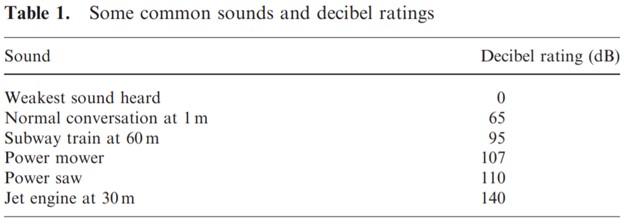
Today, logarithms are used to compare and describe natural phenomena. Logarithms are used to compare earthquakes (see Introduction), sound intensity (decibel scale), acidity, star brightness magnitude, and intensity of solar flares (Wood, 2004). Logarithms also allow us to describe radioactive decay, spread of contagious diseases, and evolution of populations (Panagiotou, 2010). Let's consider a few of these applications.Decibel Scale
Logarithmic scales are used to compare sounds. Consider the following two examples to see how logarithms are used to understand the world around us and keep us safe.
Example 1: How much more intense is a jet engine than a subway train?
 (Wood, 2005)
The equation that models sound intensity is
\(dB_2-dB_1=10log\frac{I_2}{I_1}\)
Where
\(dB=\) the number of decibels
\(I=\) the sound intensity
Where
\(dB=\) the number of decibels
\(I=\) the sound intensity
We can use this model to answer the question above.
\(140-95=10log\frac{I_2}{I_1}\)
\(\frac{45}{10}=log\frac{I_2}{I_1}\)
\(10^{4.5}=\frac{I_2}{I_1}\)
\(31,623I_1=I_2\)
\(\frac{45}{10}=log\frac{I_2}{I_1}\)
\(10^{4.5}=\frac{I_2}{I_1}\)
\(31,623I_1=I_2\)
The sound of a jet engine is 32,000 times more intense than a subway train!
Example 2: "Exposure to loud noise can cause hearing loss, so health and safety regulations limit the number of hours of exposure to noise. The Occupational Health and Safety Authority (OSHA) standard permits exposure to 90 dB sound levels for 8 hours, but if the loudness is 92 dB the exposure permitted is only 6 hours. How much louder is the 92 dB noise? (Wood, 2005)"
Based on these standards, it is interesting to note exposure to a subway train for more than 6 hours could damage our ears (see table above). This is also the reason headphones sometimes give warnings when the volume is turned up beyond a certain point.
Let's use the decibel scale model to answer the question.
\(92-90=10log\frac{I_2}{I_1}\)
\(\frac{2}{10}=log\frac{I_2}{I_1}\)
\(10^{0.2}=\frac{I_2}{I_1}\)
\(1.58=\frac{I_2}{I_1}\)
\(1.58I_1=I_2\)
\(\frac{2}{10}=log\frac{I_2}{I_1}\)
\(10^{0.2}=\frac{I_2}{I_1}\)
\(1.58=\frac{I_2}{I_1}\)
\(1.58I_1=I_2\)
A 92 decibel sound is 1.6 times as loud as a sound that is 90 decibels.
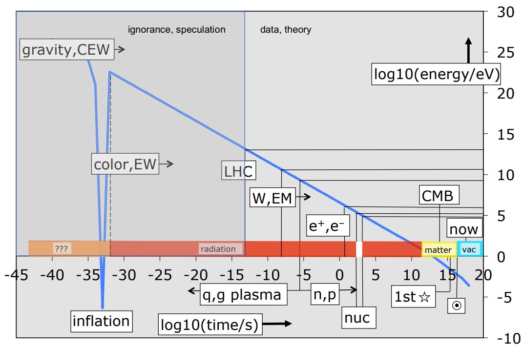
History of the Universe
For years, physicists have been trying to understand how the universe was created and why matter has certain properties. They have discovered that the universe is over \(10^{20}\) seconds old! Physicists theorized about the time frames when gravity, the strong and weak force, electrons \((e^-)\), positrons \((e^+)\), the cosmic microwave background (CMB), and many other properties of matter were introduced into our universe. Amazingly, they can summarize all these ideas on one graph using logarithms!
 (Peak, 2021)
Both the \(x\)- and \(y\)-axis of the graph are logarithmic scales. The \(x\)-axis represents time in seconds since the inception of the universe. Physicists speculate gravity was introduced into the universe \(10^{-35}\) seconds after its creation. Electrons were born roughly \(10^2=100\) seconds after the creation. The first star did not appear until roughly \(10^{16}\) seconds or over 300,000 years into our universe.
The \(y\)-axis is a logarithmic scale the represents the amount of energy in the universe. Remember the power of a logarithmic scale when comparing intensities as seen in both the earthquake and decibel examples. The energy in the universe now is hundreds of billions times less than it was when the electron was created. (Peak, 2021)
Covid-19 Models
The spread of contagious diseases are often modeled using exponential and logarithmic functions. Since Covid-19 is still a relatively new disease, the mathematical models for its spread are still being developed. Here are a few.
\(K=\frac{d(log_2 I)}{dt}\)
Where
\(K=\) Growth Rate
\(I=\) Number of Infectious People
Because the base is 2, \(\frac{1}{K}\) predicts the amount of time it would
take for the number of infectious people to double (Konishi, 2021).Where
\(K=\) Growth Rate
\(I=\) Number of Infectious People
\(B(t)=C_B*log(N-I(t))\)
Where
\(B(t)=\) "number of individuals taking measures to resist the virus-propagation while being completely confined" (typically in the millions)
\(C_B=\) A Proportionality Constant
\(N=\) Total Population in a Country
\(I(t)=\) "number of infected individuals who can move freely" (typically in the thousands) (Abdalla et al., 2021)
This equation is a steppingstone toward building a more complex mathematical model which includes imaginary numbers.