The content of this page is centered on the topic of complex numbers. This page will walk through the history of complex numbers. It will discuss the mathematical discovery, how we got the name, and the research that is continuing today. It will talk about the math that lead to its discovery and what it means. It will teach about the basics of how we use compute complex numbers and its properties. It will also talk about the application, The Mandelbrot Set and its significance.
This is a topic that has fascinated me from the moment I first learned about it. My experiences in studying the topic have lead to a greater knowledge and appreciation. As you explore this website I hope you too will learn something new that you find exciting.
Complex numbers were found and used long before they were defined. Thus, it is hard to find an exact beginning. However, it wasn’t a discovery that initially provoked a lot of excitement. For decades, mathematicians played around with the idea without much conviction. In fact, many rejected the concept. Mathematicians initially called them “fictitious numbers;” which, later evolved to the name imaginary numbers that we know today. The question is: are they real? Do they exist? Why did mathematicians use complex numbers if they didn’t think they were ‘real?’ Well these answers come with a fascinating story.
The history of complex numbers is often compared to that of negative numbers. Today we know that negative numbers are real and very useful in mathematics. Negative numbers explain debt or overdrawn accounts in banks and businesses. We use them to represent temperatures, direction and so much more. With how common negative numbers are and our many uses for them now it is easy to see how real they are. However, it wasn’t always so clear. There was a time with mathematicians argued whether they were real or whether you could really use them mathematically. The same thing happened with complex numbers.
Though complex numbers were found and seen for hundreds of years it became somewhat of a stopping point for many people. One of the most recognized ways mathematicians continued to see imaginary numbers pop up was in their quest to solve polynomial equations. The solution to quadratic equations extends across the world and over 4,000 years. The earliest solution found was by the Babylonians in 1600 BCE. However, even with many solutions popping up most simply thought the equation broke when they saw √(-1), which makes sense.
Quadratic Equations
The image to the left is an example of a quadratic equation graphed on the Cartesian plane. The equation y=x2-x-2 has two solutions. In other words, it crosses the x-axis twice or has two roots. This is a very simple graph with very clear solutions of -1 and 2. The problem found when finding solutions to quadratic equations was not when it crossed the x-axis, but when it didn’t.
The image to the right is an example of a quadratic equation where the graph doesn’t cross the x-axis. From this image it makes sense that mathematicians believed there just wasn’t an answer. Mathematically when they tried to solve a quadratic equation that didn’t cross the x-axis they would find imaginary numbers, meaning √(-1). Therefore, when mathematicians saw √(-1), they didn’t believe it to exist. Additional explanation of the math behind the example to the right can be found here .
Cubic Equations
What finally made mathematicians begin to use imaginary numbers was the discovery of the solution to cubic functions. Now, at the time mathematicians would compete in duals for prestigious math positions. When a mathematician believed they could win, they would challenge a mathematician that had the position they wanted to a dual. Both would create a list of problems they knew how to solve and give it to the other. Whoever completed the problems first would win and thus get the position. This created an environment where mathematicians kept their research very quiet. They didn't want their opponents to know what they knew.
This also makes it hard to give credit to a mathematician for discovering different formulas. For example, one equation that several mathematicians discovered and used in duals was a formula to solve cubic functions. This formula was taken to the grave by several mathematicians before it was even known by most of the mathematical world. What was so significant about the solution to this problem was when solving cubic functions several mathematicians had to work through complex numbers. Below is the modern notation of the solution that was discovered.
This formula forced mathematicians to use imaginary numbers. However, even mathematicians that used the formula at the time didn't think imaginary numbers really existed. They believed they were just necessary to use for some computations. Then came the famous mathematician, Gauss. In 1799 Gauss came up with the first proof of a theorem so important it is called The Fundamental Theorem of Algebra.
The Fundamental Theorem of Algebra states that for every polynomial of the nth degree there are n roots.
This theorem gave credibility, proof of existence and purpose to imaginary numbers. For more information click here or here .
Since then, mathematicians continue to study complex numbers and the existence of them. In fact, today, there are even several methods to explain how we can visualize imaginary solutions. The basic idea is that imaginary numbers exist on a different plane. Meaning, we can't see the solutions because we are not looking in the right place. For deeper explanations the following links will take you to two different articles. Click here or here .
My favorite explanation of how we can visualize complex roots can be explored through this Geogebra applet.
Visualizing Complex Roots of Quadratic Equations
Now we know, not only do they exist, but imaginary numbers are also very useful. Now there is a general consensus that imaginary numbers are unfortunately named as they do exist and are not imaginary in any way. In fact many people today believe that the name imaginary numbers is what is so confusing about them. Students learning about them tend to get hung up on the name 'imaginary' more than the concept its self.
What is a Complex Number?
The image to the left gives a visual representation of the different types of numbers. Lets start by remembering what real numbers are. Real numbers consists of natural numbers, whole numbers, integers, rational and even irrational numbers. Outside of the real numbers there are what is called imaginary numbers.
Now, as mentioned above, the names aren't perfectly named. The names real and imaginary don't imply that the real numbers exist while the imaginary numbers are just imagined. Both types of numbers exist.
Complex numbers simply incorporate the two numbers. Every complex number has two parts. It has a real part and an imaginary part. The image to the right shows how complex numbers are written. "a" is the real part, "b" is the imaginary part and "i" is √(-1).
The symbol i is defined as √(-1) where i2= -1.
Graphing Complex Numbers
As discussed, in the history of complex numbers, mathematicians saw imaginary numbers as a place where the system broke. However, when they realized that they did in fact exist there came about the question: where are the complex numbers? How do we represent them graphically?
The arithmetic was clearly defined: Multiplying 1 by i2 results in -1. The challenge was, how to graphically represent two values multiplied together to get from 1 to -1. The solution became a rotation. The rotation to the imaginary axis, or another plane.
This different dimension created a new plane. It created the complex plane. On the complex plane the imaginary numbers had their place. Visually it is like the Cartesian plane. The difference is that instead of it being the y-axis it is the imaginary line and instead of the x-axis it is called the real number line. Thus, we could graph complex numbers.
Just above we see an example of a complex number graphed on the complex plane. As stated above, every complex number has both a real part and an imaginary part. The real and imaginary number lines give a place for the complex number to be graphed. Looking at the example 3+2i: we move in the positive direction on the real number line 3 units. Then we move in the positive direction on the imaginary number line 2 units. The end point represents the complex number graphed on the complex plane.
Powers of Imaginary Numbers
Using this definitions there are simple rules we can follow to simplify the powers of i.
i1= √-1, i2= -1, i3= -√-1, i4= 1
After these first four powers the pattern starts over. This means that if you divide the power by 4 then the remainder tells you what the solution should be. For example, if you divide the power by 4 and the remainder is 1 then the solution is √-1. If you divide the power by 4 and the remainder is 2 then the solution is -1. If you divide the power by 4 and the remainder is 3 then the solution is -√-1. If you divide the power of i by 4 and there is no remainder, then the solution is 1.
The picture on the right shows the graphical representation of the powers of i. The challenge of visually understanding imaginary numbers is described above. However, this picture does a wonderful job of reflecting the solution. The rotation 90 degrees to the imaginary number line creates a 'midpoint' between the numbers 1 and negative 1. As we continue to multiply by i we can see how it rotates around the graph in a counter clockwise fashion. This is a distinct property of the complex plane that is useful in trigonometry and the arithmetic of complex numbers.
For now, if you are looking for more information about the powers of i click on the video to the right. The video is a detailed explanation of the mathematics as well as a different perspective of understanding. It also goes through several examples. This is a great video to learn about the powers of complex numbers.
Arithmetic of Complex Numbers
The arithmetic of complex numbers is very simple. We treat complex numbers the same way we treat variables. Below are two images that demonstrate how we preform addition and subtraction on complex numbers. Treating i like a variable we simply add or subtract like terms. In the bottom right corner of the two images below is how the simple x variable relates to the simple arithmetic of adding and subtracting imaginary numbers.
The multiplication of complex numbers is similar to addition and subtraction in that it follows the rules of a variables. For example if we were multiplying the following expression (2+x)(3-4x) we would foil and then add like terms. In a similar way we foil complex numbers. The image to the right gives a colorful representation of how to foil complex numbers. Then once the complex numbers are foiled we simply add like terms. The key difference is that with the example with the x variable we will find x2 appear in the solution. However, we know that i2= -1 by definition. Therefore, when we multiply the "outers," that value becomes -bd. This makes it a like term to the "firsts" or the value ac after foiling. In the end there will be two real numbers to combine and two imaginary numbers to combine to create a new, multiplied complex number.
Lastly there is the division of complex numbers. The first step to dividing complex numbers is simply writing the complex numbers in fraction form. The second step is to multiply both the top and bottom of the fraction by the complex conjugate of the denominator.
The complex conjugate is defined as follows. If a complex number is a+bi the complex conjugate is a-bi. If a complex number is a-bi the complex conjugate is a+bi. It is as simple as that.
To multiply the numerator and the denominator by the complex conjugate, follow the rules of multiplying complex numbers. In the example to the right we see why we multiply the numerator and the denominator by the complex conjugate. The multiplication of the numerator results in a new complex number. However, the multiplication of the denominator results in just a real number. From there it is easy to combine like terms and see that the result is a complex number in the form a+bi.
Graphically representing Complex Arithmetic
Lets start by simply looking at the real number line. To the right is an explanation of how we would graphically represent addition and subtraction of real numbers on a real number line. The idea is to use vectors with the magnitude of the number. The first vector starts at the origin and reaches to the value. The second vector starts at the tip of the first. If both are positive they both point in the positive direction. If both are negative, both vectors point in the negative direction. However, you can also say one is negative and one is positive. Every variation works as long as the vectors are the magnitude of the value and it is in the correct direction. The solution them becomes a new vector that start at the origion and ends at the tip of the second vector.
The same idea can be used with the two dimensional complex numbers. The image to the right shows an example of graphically representing addition on the complex plane. It also shows how it compares to the numerical arithmetic of adding complex numbers. Visually the image below is a wonderful representation of how graphically addition is still commutative.
No matter which of the two vectors you start with you will end up at the same result.
Subtraction is very similar as well. Below is an image that graphically shows addition (on the left) and subtraction (on the right.) This image makes it very easy to compare and see the differences. Just as in our example with the real numbers, if we are subtracting the number it needs to be pointed in the negative direction. On the real number line this is very easy to visualize. On the complex plane it can be a little more difficult. However, the idea is the same!
In the graph on the left we see the addition of z1 and z2 to get the yellow vector. This is just using the addition method we discussed above. On the right we simply drew a new vector showing z2 in the 'negative direction' or the negative of the vector z2. Then, we simply add the negative of z2 and vector z1 to get the subtraction of the two vectors. This is equivalent to the algebraic idea of a minus b is the same thing as a plus the negative of b, or b in the negative direction.
Now to explain the graphical representation of the multiplication of complex numbers I created a Geogebra applet. All explanations of how it works and its significance can be found when you click on the link below.
Exploring the Multiplication of Complex Numbers Graphically
To understand one of the applications of complex numbers and its significance, we first need to have a basic understanding of fractals.
Fracals
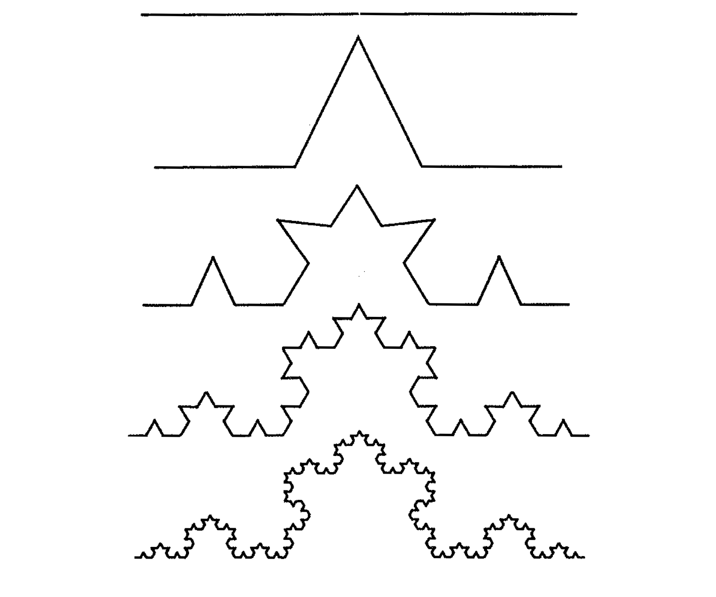
Let's start by looking at the picture to the right. The pattern starts with a basic line. Then we break that line at he midpoint and create two lines. The two lines can be described as two sides of an equilateral triangle. The third line, the base of the equilateral triangle, is not drawn. This creates four lines, where, in the stage before there was only one line.
Now, looking at the second row we have four lines. To continue this same pattern, we do the same thing we did above. This time we simply have more lines to do it with. As we see, moving from row two to row three results in eight more lines. In row three, we now have a total of sixteen lines to continue the pattern.
In the image the pattern repeats for rows four and five. Each row results in more lines. However, it doesn't have to stop there. In theory the pattern continues forever. Mathematically, this creates an infinitely long line.
Instead of starting this pattern with a line, we can start it with an equilateral triangle. An animated picture of this is located to the left. It starts with an equilateral triangle and shows what the first few iterations look like.
This is called the Koch Snowflake
The Koch Snowflake has a unique property. It is created using a simple pattern, iterated over and over. Therefore, no matter where you look or how much you zoom in, you will see the same pattern over and over. In other words, it is created to be a never ending pattern. Never ending patterns, like this, are called fractals.
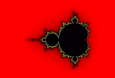
One of the most recognized fractals is known as The Mandelbrot Set.
The Mandelbrot Set
The Mandelbrot Set is created using a simple equation repeated over and over. In other words, it is the iteration of an equation. Let's start with a simple example on the real number line. We will start with the numbers 0-5. The equation we will use is zn= zn-12. First, I will state that z1 = 0. The first few iterations are as follows: z2 = 0, z3 = 0, z4 = 0, and so on. Of course squaring the number 0 will always give the result 0. The number 1 is very similar. If z1 = 1 then we will get similar results: z2 = 1, z3 = 1, z4 = 1, and so on. This is because no matter how many times you multiply 1 by its self, the result is always 1. The numbers zero and one are examples of the first possible outcome of this equation under this iteration: the result is bounded. This means that no matter how many times you do iterate it, the solution will always have a finite limit.
Now, let's say z1 = 2. The first few iterations are as follows: z1 = 2, z2 = 4, z3 = 16, z4 = 256, z5 = 65,536, and so on. In the case where z1 = 2, the iteration results in a number that gets large very quickly. Now, let's say z1 = 3. The first few iterations are as follows: z1 = 3, z2 = 9, z3 = 81, z4 = 6,561, and so on. Now, let's say z1 = 4. The first few iterations are as follows: z1 = 4, z2 = 16, z3 = 256, and so on. Our last example is z1 = 5. The first few iterations are as follows: z1 = 5, z2 = 25, z3 = 625, and so on. These are examples of the second possible outcome of this equation under iteration: the result goes to infinity. This means that with many iterations the number will just get larger and larger until it is uncountable.
What is interesting to note is the differences in the four examples of second possible outcome. After the first iteration for the starting points four and five most people would need a calculator. However, starting with the numbers two or three the average person is more likely to make it to the second iteration before needing a calculator. Thus we see that these numbers get bigger at different rates. This idea is crucial to understanding The Mandelbrot Set.
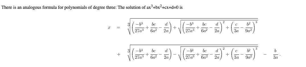
The equation of The Mandelbrot set is slightly more complicated. The equation is:
zn= zn-12 + c , z1 = 0
The last piece of the puzzle you need in order to understand The Mandelbrot set is that it exists on the complex plane. So far we have only been working on the real number line. What makes the complex plane so interesting is that it brings another dimension.
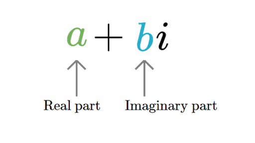
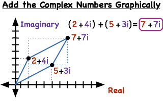
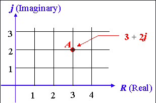
Complex numbers have two parts: they have a real part and an imaginary part. Thus, graphically we represent a complex number as a two dimensional number. In the picture to the right we see that A is a two dimensional number.
The Mandelbrot equation on the complex plane has the same two possible outcomes:
Under iteration the result is either bounded (Stable), or it goes to infinity (Unstable).
To summarize, The Mandelbrot Set is created by the iteration of the equation zn= zn-12 + c. In The Mandelbrot Set, z1 is always equal to 0. Under iteration the result behaves one of two ways. It either is bounded (in other words: stable) or it goes to infinity (meaning unstable.) The Mandelbrot set exists on the complex plane, using two dimensional numbers. By hand all of these new factors are hard to visualize. To further explore what is Stable and Unstable on the complex plane iterating the Mandelbrot equation click the button below. This will take you to a Geogebra applet that calculates the first 200 iterations of the Mandelbrot equation for any value of c. Notice how the patterns relate to the image of the Mandelbrot set.
If you still are not impressed with what you have found in the applets, click on the image to the right. This is a link to a video that zooms in on The Mandelbrot Set for over five minutes. It is calculated using 750 million iterations!
What is the Significance?
Mandelbrot famously wrote: "Clouds are not spheres, mountains are not cones, coastlines are not circles, and bark is not smooth, nor does lightning travel in a straight line."
For a long time people only studied regular shapes like spheres, cones and circles. However, there are so many things that can't be described with these basic shapes. Fractals are what connects the simple to the chaos. Fractals give us a way to explain and study irregular, chaotic things. Fractals are a way to model what we could never model before. It is a new mathematical way to study the world. With fractals we can measure coastlines more accurately, we can mathematically create realistic virtual realities, we can begin to understand the common irregular things in the world around us.
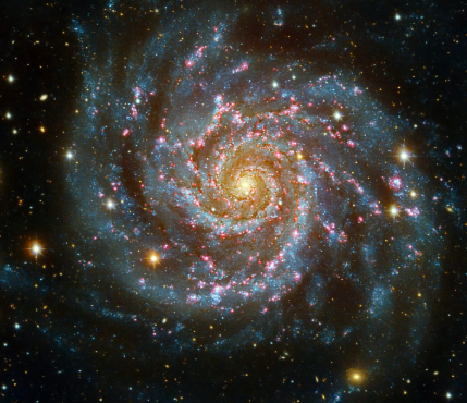
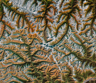
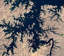
Fractals found in Nature
Adams, G. (2015, Nov). A brief history of quadratic equations for mathematics educators. Retrieved from British Society for Research into Learning Mathematics: https://bsrlm.org.uk/wp-content/uploads/2016/02/BSRLM-IP-35-3-16.pdf
Christersson, M. (2015, December). Animate Julia Sets. Retrieved from Malin Christersson: http://www.malinc.se/m/JuliaSets.php
Dabbs, M. (2019). Complex Iteration - The Mandelbrot Set. Retrieved from Geogebra: https://www.geogebra.org/m/tEetDqXF
Fractal Universe. (2017, July 7). The Hardest Mandelbrot Zoom in 2017. Retrieved from YouTube: https://youtu.be/aSg2Db3jF_4
Glancy, A. (2019). Visualizing Complex Roots of Quadratic Equations. Retrieved from Geogebra: https://www.geogebra.org/m/U2HRUfDr
Hanson, A. J., & Sha, J.-P. (1998). Exploring Visualization Methods for Complex Variables. Retrieved from Computer Science Department and Mathematics Department Indiana University: http://citeseerx.ist.psu.edu/viewdoc/download?doi=10.1.1.402.7156&rep=rep1&type=pdf
Numberphile (Producer), Haran, B. (Writer), & Haran, B. (Director). Fundamental Theorem of Algebra [Motion Picture].
Hobart and William Smith Colleges. (2019). Explore the Mandelbrot Set. Retrieved from http://math.hws.edu/eck/js/mandelbrot/MB.html
Jackiw, N. (2003, Oct). Visualizing Complex Functions with The Geometer’s Sketchpad. Retrieved from Proceedings of the 6th International Conference on Technology in Mathematics Teaching. : http://citeseerx.ist.psu.edu/viewdoc/download?doi=10.1.1.729.5162&rep=rep1&type=pdf
Khan Acadamy. (2011). Powers of the imaginary unit. Retrieved from Khan Acadamy: https://www.khanacademy.org/math/algebra2/x2ec2f6f830c9fb89:complex/x2ec2f6f830c9fb89:imaginary/v/calculating-i-raised-to-arbitrary-exponents
Khan Acadamy. (2016). What is a fractal (and what are they good for)? Retrieved from Khan Acadamy: https://www.khanacademy.org/partner-content/mit-k12/mit-math/v/what-is-a-fractal-and-what-are-they-good-for
Math is Fun. (2017). Fundamental Theorem of Algebra. Retrieved from Math is Fun: https://www.mathsisfun.com/algebra/fundamental-theorem-algebra.html
Peters, C. (2018). The Reality of the Complex: The Discovery and Development of Imaginary Numbers. Retrieved from Lee University: http://sigmaa.maa.org/hom/resources/Contests/Peters2018.pdf
Roberts, D. (2019). Quadratic Equations with Complex Solution. Retrieved from Math Bits Notebook: https://mathbitsnotebook.com/Algebra2/Quadratics/QDQuadratics.html
Schechter, E. (2013, Jan). The Cubic Formula. Retrieved from Vanderbilt: https://math.vanderbilt.edu/schectex/courses/cubic/
Schwartz, R. (2014, Oct 1). The Fundamental Theorem of Algebra. Retrieved from Brown University: https://www.math.brown.edu/~res/INF/handout5.pdf
Windred, G. (1929, Oct). History of the Theory of Imaginary and Complex Quantities. Retrieved from The Mathematical Gazette: https://www.jstor.org/stable/3606116?origin=crossref&seq=1#metadata_info_tab_contents