People all over the world have predicted cataclysmic, human extinction, global
events for hundreds of years.
From Halley’s Comet in 1910 that was supposed to trigger an apocalyptic explosion
to the Y2K bug when computers would cause the collapse of civilization in 2000
to the Large Hadron Collider creating a black hole with its particle accelerator that would swallow the earth in 2008
to the Mayan calendar predicting the ‘end of the world’ in 2012
and many others. (Lakritz 2019)
In fact, there is a whole Wikipedia page dedicated to times people thought the world
was going to end! (Wikipedia 2022) On this page, there are 178 listed past predictions
of the world ending and 16 predictions of it happening in the future, 3 of them in the
near future.
Although the world hasn’t ended yet, who’s to say it won’t eventually?
If there are so many people predicting the end, doesn't that mean it will come?
If it does happen during our lifetimes, we are going to want to be able to
accurately predict how many animals we will have and how many we can eat.
Many people have small farms with some animals on them and, if the world is going to end,
we want to be able to predict the amount of animals we will have in the apocalypse.
The best way to visualize this is through
mathematical modeling.
Mathematical Modeling
According to Katie Kavanagh and Ben Galluzzo (2022), “Mathematical modeling refers to the
process of creating a mathematical representation of a real-world scenario to make a prediction
or provide insight.”
That is exactly what we are doing with our animals in the apocalypse!
We want to create a representation of a real-world scenario when the world ends to make a
prediction of how many animals we will have.
History of Mathematical Modeling
The history of mathematical modeling is hard to find, because mathematical modeling is so broad.
Mathematical models come in many different forms.
There are
equations
graphs
tables
diagrams
physical models
and more!
For this project, we could probably use all of these. But, we are just going to focus on a few.
The most helpful models are going to be equations and graphs.
It is important to note that because there are so many different types of mathematical
models and so many different applications for them, the history of them could be different
for the different applications. It would take multiple books to research and compile
the complete history of mathematical modeling.
Brief History of the Mathematical Model: Equations
Math for a long time was just used for counting and looking at relationships between shapes.
That was all that it was needed for. But, sometime during the 1600s that started to change.
Math started to grow like crazy, and that is mostly because of equations. Most of us
have seen equations in our lives. We have used them in school over and over again and, believe it or not,
we use them all the time in our daily lives. An equation is something with two sides that equal eachother.
Once people started to understand equations, they found amazing ways to apply them. Equations
are everywhere and can be used for everything. Enclycopedia.com says,
"By introducing systems for accommodating variables and unknowns,
and the tools for solving those items, the equation became a powerful mathematical
tool, with applications that reached far beyond the realm of numbers, affecting
everything from construction (geometry) to theories of the motions of the planets
(calculus) and embracing virtually every field of human endeavor." (Ferrell)
Although equations were used long before the 1600s, (as far back as the Ancient Greeks in 1200 BC),
there needed to be rules and standardization in order for them to become what they are today.
A few of the people that made important progress and what they did are listed below. (Information from Ferrel)
Diophantus of Alexandria
He is known as 'the father of algebra.' Before him, equations were written in words.
He was the first to use symbols in equations. He would use Greek letters
to represent amounts that were used often. Because of this, equations became
easier to create and solve.
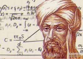
Muhammad ibn Musa Al-Khwarizmi
He translate the work of Diophantus and developed it further in a book he called
"Al-jabr." The modern name of 'Algebra' came from this book. On top of
naming algebra, Muhammad also incorporated some concepts from Hindu sources.
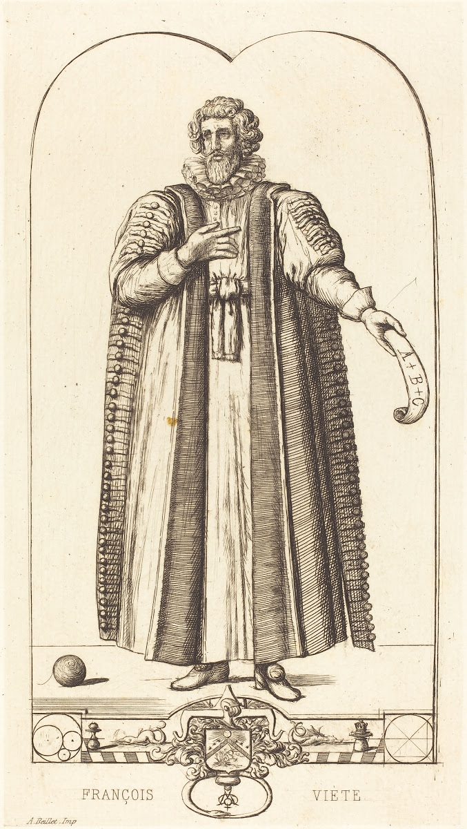
François Viète
François was the first to use letters of the alphabet in equations.
He used them to represent unknown variables and constants. He would use
vowels to represent the unknown variables and consonants to represent the
known variables. This was a big step for algebra.
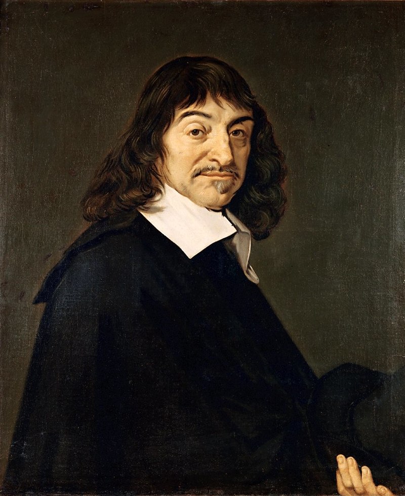
René Descartes
Descartes worked with what Viète came up with and focused it even farther.
He used the letters at the beginning of the alphabet as symbols for numbers,
and letters at the end of the alphabet as symbols for variables. It is because
of his work that we are so used to x and y in algebra.
Brief History of the Mathematical Model: Graphs
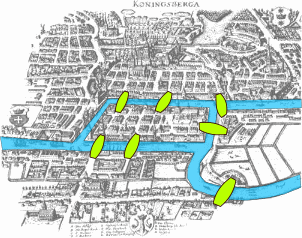
The history of the graph starts in Königsberg, Prussia in 1735.
Below is a picture of the city. There were 4 land masses separated by water.
There were bridges from each land mass to the ones next to it as shown.
There was a fun riddle that the people who lived there would try to figure out.
Could a person walk on each bridge without using a bridge twice?
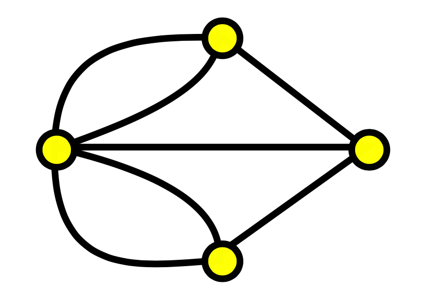
A very famous mathematician, Leonhard Euler, is the one that ultimately solved this problem.
And he did it using a graph, the first graph.
He created the graph below, where the points represent the different land masses,
and the lines represent the bridges.
Using this graph, Euler proved that you could not walk on every bridge without using
one twice. He proved that in order for a problem like this to work, each point would
need to have an even number of lines coming from it. (Laurenti)
Since then, many graphs have been made and expanded and learned from.
Mathematical Modeling Process
The mathematical modeling process is a cycle. There are 6 steps, but you cycle through
them as many times as you need to get the best model. The steps are the same no matter
where you look, they are just stated using slightly different words. According to Anhalt
and Cortez (2015) the steps are:
Analyze a situation or problem
Develop and formulate a model
Compute solution of the model
Interpret the solution and draw conclusion
Validate Conclusion
Report the solution.
The cycle occurs after step 4. Instead of moving on to step 5, you go back to step 2
and continue this until you believe you have the best model.
We am going to go through the process focusing on finding a good model for pigs,
then we can use that for other animals if we want.
Step 1
For the first step in making a mathematical model for animals in the apocalypse,
we need to
analyze the situation.
We need to know how fast pigs will multiply and how many we will have in the apocalypse.
This step is super important. We have to understand what we are looking for and what we
are looking at, or the whole process with be a mess. When we analyze the situation, we
are setting ourselves up for success. If we make sure to do this step, we can focus
the rest of the steps on our situations and what we are really trying to find.
Without this step we would need to go through the process more times just to refine what
we are finding.
Step 2
The second step is
developing and formulating a model.
There are steps within this step.
Find all the given information
Take the information and translate
it into a mathematical problem that can be solved
First, we need to
find all the given information.
There are two categories of information. There is information that will change over time, and
information that will (basically) not change over time.
Information that changes over time:
How many of the animal you start with
How many are females
How old they are
How often you eat a pig
How often you sell a pig
The size of their pen
Information that will not change over time:
How long they live (on average)
How old they must be to start breeding
Gestation period
Average litter size
How many pigs survive to adulthood
How big the pig gets
How much it costs to feed a pig
How much it pays to sell a pig
How much meat you get from your pig
How much space the pig needs
Some of the information that won’t change over time will need to be assumed.
It will get really complicated if we try to make those too accurate or
change for different breeds, so we will use averages for some of the variables.
The next thing we need to do for this step is
take the information and translate
it into a mathematical problem that can be solved.
We are going to start with a
polynomial including the different variables.
t=time
a=how many animals you start with
b=how many are females
c=how old they are (on average)
d=how often you kill a pig to eat
e=how often you sell a pig
f=the size of their pen
g=how long they live (on average)
h=how old they must be to start breeding
i=length of gestation period
j=average litter size
k=how many pigs survive to adulthood
l=how big the pig gets
m=how much it costs to feed a pig per month
n=how much it pays to sell a pig
o=how much meat you get from your pig
p=how much space each pig needs
As you can see, this is a lot of variables and a lot of information.
It could actually make a few different equations:
How many animals at a certain time (q(t))
q(t)=(a-b)+(b*jk^t/i)
How much money you have spent/made this month (r(t))
r(t)=(n*e)-(m*q(t))
How much meat you have (s(t))
s(t)=(o*d/t)-how much meat you have eaten
As you can see, there are a lot of variables here.
These variables were all brainstormed. First we thought of step 1 where we looked at our situation. We
thought of the variables that we want to know. Then we though of all the variables that we already know
that could possibly help us figure out the variables we want to know. Lastly, we thought of all the variables
that we don't know yet, but we will need to know in order to figure out our variables we want to know.
This list is not all of the variables possible, but after sorting through the list multiple
times this is what we ended with. We went through a process of elimination.
First we had a very long list of every variable we could think of that could be related to our situation.
Next we went through this list and got rid of variables that would make this model more complicated
than we wanted.
These are the variables we got rid of, and why:
How often the pigs get sick
We got rid of this because it would be very complicated to add into the model
the chance that a pig gets sick. This would change depending on how old the pig is, and would
make it unneccesarily conmplicated because the average life expectancy would essentially take
care of this.
How often the pigs run away
We got rid of this for a very similar reason as the variable above. It would be
complicated to add in the chance that the pig ran away, when it will be low anyways if we have a good
enough fence.
How often people steal pigs from us
Again, this is very similar. It won't be large because of the fence of the pigs. It would
be complicated and unnecessary for the model we want. We don't need a model that is exactly accurate,
we just want an idea of how many animals we will have over time.
The chances that the pif dies earlier/later than average
This one is pretty applicable to the problem we are focusing on, but it is rather complicated.
We already have a variable that is the average life expectancy for the pigs, so to add in this chance would
be to replace that variable. This would be hard because we would need to do the chance process for each pig
each year to see if it will continue to live. It could be interesting to add, but it would be
extremely complicated. Therefore, we decided to elimate this variable. If in the future we decided
to continue developing this model further to make it more complicated and accurate, this would be a good
variable to add back.
Next we went through our list of variables and enacted another process of elimination. This time we
got rid of variables that seemed to be unhelpful towards our end result.
The variables that were elimated this time and why were:
Different breeds of pig
This is relatively unimportant. The different breeds of pigs have very little differences
in all of the variables we are focusing on. To keep this variable would to just add confusion. It doesn't
add to our problem or our model in any helpful way.
How many of the pigs are male
When we were first deciding variables, this was one of the first that was written down.
As the process continued though, we came to the realization that it has no substance whatsoever. We already
have a variable that is the total number of pigs, and we have a variable that is the total number of females (because we need
to know how many can have babies), thus this variable is redundant. Instead of this, we can just do the total
number and subtract the total females.
How much pig feed costs
We realized that this variable doesn't add to our model. We aren't focusing on how much
money we will have or spend, so we don't need to know how much a bad of food costs. We also already have
the variable that is how much it costs to keep the pigs for a month, which would contain this. There is no
need for it to be separate.
This is why the first step was important. We had to know what we were working with and what we were
focusing on so we could know what variables are possible and what variables we want to focus on.
But, even with the first step, we changed our list of variables multiple times, and still don't believe
it is the best list we could have ended up with.
Each situation has different variables and a different requirement for precision. Some mathematical
modeling processes will be very simple while others can be extremely complicated. This is another reason
why the first step is crucial. Without that step, the second step cannot be done properly.
The equations/models that were created were done so using the variables that
we found and trying to guess the relationships they would have with eachother.
For the number of animals we thought we could take the number of males, and add the number of females multiplied by
how many babies they would have each year.
For the amount of money you have spent/made this month we thought you could just multiply
how much it pays to sell a pig by how many you sell and subtract how much you spent on the pigs.
For how much meat you have all you would need to do is multiply how much meat you get from each pig
with how many pigs you kill to eat.
As you can tell, this step is rather complicated. This is one of the biggest steps of the process.
You have to take all of the information you know, and change it to make it into a model.
For most people, it would make sense that this is the only step in make a mathematical model, actually making it.
BUT
That is not the case. This is definitely not the end of the modeling process. As you continue to read, you will
see how incomplete our model would be if we stopped right here.
Step 3
Now I need to compute the solution of the model.
In order to do that, all I do is plug in the numbers to my equations.
I am going to compute the solution for each of the equations after 1 year. We will start with a hypothetical farm of
2 female pigs that are old enough to breed and 1 male.
If we plug in the numbers to q(t) we get:
q(1)=(3-2)+(2*7*.8)*(1/.3)
=38 pigs
If we plug in the numbers to r(t) we get:
r(1)=(n*e)-(75*38)
We can't solve this equation because we don't know how much we will get
paid to sell a pig in the apocalypse, nor how often we would sell them.
If we plug in the numbers to s(t) we get:
s(1)=(.75)*d/1
We can't solve this one either because we don't know how often we want to kill a pig
to eat it.
This step is a little bit easier than step 2 because all you have to do is plug in the
numbers you already have. This step is important so we can interpret it and draw conclusions in the
next step.
Below you can see all of the models we just looked at.
Step 4
Now it is time to interpret the solution and draw conclusions.
For the model of q(t) it has a positive linear slope, and told us we will have
38 pigs after one year.
This tells us that the number of pigs is growing, but always at the same rate.
This may be a good model to start with, but definitely not the most accurate.
It is also important to note that it told us we would have 38 pigs after one year.
Maybe this is possible, but it seems relatively unrealistic that a female pig
would have two litters of pigs each year.
If we were to redo this model, we might think about changing the relationship between
variables. Just because their gestation period is 3 months, doesn't mean they will have a
new litter every 3 months.
For the model of r(t) we can't even solve it. It isn't what we wanted to focus on in step 1,
and it is hard to estimate.
If we were to redo this model, it may be best to get rid of it.
For the model of s(t) it is similar to r(t). We can't solve it, and it isn't what we are focused
on in step 1. It may be important to know in the apocalypse or interesting to know now, but
it isn't what we are focused on. If we were to redo this model, we should probably get rid of it as well.
This step is important because we are applying our model to real life and deciding if it
makes sense. We are checking what we have done so we can see if we need to make changes.
What we do is take our answers from step 3, and we think about them in context. If it makes sense,
that's great! If it doesn't, we need to think about why and what we can do to fix that.
In this case, the first model made the most sense. It could work in real life, but there
are definitely some adjustments that should be made. This wouldn't be a model you would want to
rely on.
For the other models, we realized we didn't even need them at all. It is a good thing we had this step,
so we could realize that and make the change.
Step 5
Now we need to
validate our conclusions.
We don’t want to look at multiple models. Although r(t) and s(t) would be cool to know,
that is not what we want to know and what we specified in step 1.
We are going to want to adjust the variables accordingly.
We may also want to change the variables to all be in terms of months,
so it is uniform and easier to work with in the models.
The linear growth made sense because it was growing, but not realistic.
Now it is time to cycle through the modeling process again.
This step is important because it prepares us to cycle through the process again.
We applied what we saw in step 4, and decided to get rid of the extra models that we aren't
focusing on right now. We also looked at the first model, and thought of ways we could make it better.
We could go through this process over and over until we found the perfect model.
By following this process, we can make sure we are always moving towards finding a better model
and finding a model that we want to use to find the variables we want to know.
The cool thing about this process is how personalized it can be for each problem we work with.
No matter what you are trying to make a model of, this process will work for it. If you do each step
thoroughly, you will end up with a model that gets you what you want. It takes time, work, and a lot of
revising, but you will get there.
Some Models
So you can see some other models, we went through the process a couple more times. Following
are some of the models we came up with and their respective variables and changes from the previous models.
Model #2
Changes in Variables:
c=how old they are in months (on average)
Removed the variable "d=How often you kill a pig to eat"
Removed the variable "e=How often you sell a pig"
g=How long they live in months (on average)
h=how old they must be (in months) to start breeding
How long their gestation period is (in months)
Removed the variable "m=How much it costs to feed a pig per month"
Removed the variable "n=How much it pays to sell a pig"
Removed the variable "o=How much meat you get from your pig "
We decided the rate of growth can be shown as
u(t) = b*(t/i)*j*k
and the population formula would be
P(t)=p0*e^(u(t)*t)
Final Model
Changes in Variables:
t=time in months
a=how many males you start with
b=how many females you start with
c=the size of their pen/space in square feet
d=how long they will live on average in months=198 months
e=how often a pig will have a litter=1/12
f=average litter size=7
g=how many pigs survive to adulthood=.8
h=how much space each pig needs=8 square feet
m(t)=male pigs after t months = a + b(t) * .5
f(t)=female pigs after t months = b + b(t) * .5
b(t)=baby pigs after t months = b * (t/(e)) * f * g
p(t)=total pigs after t months = f(t) + m(t)
s(t)=space left for pigs = c - (h * p(t))
Where p(t) < s(t)
Below is an interactive applet so you can see the different models in action,
and compare them to one another.
Significance and Applications
After going through this process just a few times, we have already learned a
lot about my model and made progress.
Mathematical modeling is applicable in so many different areas of life.
Every profession uses mathematical modeling, whether they realize it or not.
Even simple graphs or simple equations are mathematically modeling whatever the
professional is working with in their work. All of these professionals are even
doing the mathematical modeling process without realizing it.
They are gathering information, creating models, and revising these models until
they make sense.
Mathematical modeling is a lot more applicable than people think.
You may be at the store shopping for socks and start using the mathematical process
without even realizing it. You may see one pack of 7 pairs of socks for $20 and
another pack of 5 pairs of socks for $14. You wonder if one of them is a better deal.
One way you can find out is by doing $20/7 pairs of socks and $14/5 pairs of socks
and see which one is less. You do this, and find out that 7 pairs for $20 is just less
per pair of socks. Then you see more pairs of socks and compare to those. This is a simple
act that most people do at the grocery store. Although they don't write out the equations,
they are going through the mathematical modeling process to find a model (or equation)
that represents the situation they are in. They may have to revisit their equation and adjust it
once or twice until they have the best one.
In science we use mathematical models all of the time, and use the modeling process just
as often. There is almost nothing you can do in any branch of science without
come kind of mathematical model. We can't work with molecules and ions if we don't
have formulas that tell us how they work together.
We can't calculate force or work in physics if we don't have the equations to do so.
We can't learn about different parts of biology and other sciences without graphs, tables,
and models.
Mathematical modeling and the mathematical modeling process is crucial to businesses
and entrepreneurs. They need to know things like revenue, marginal revenue, maximizing profits,
profit margins, demand, etc. They use equations to find out if their business is going to be successful
and to assess how they are doing and how they can do better.
Every one of those equations they use is a mathematical model, and they go through the mathematical modeling process
to find the equation that does the thing they are looking for and tells them what they need to know.
Mathematical modeling is absolutely crucial to statistics. It is most of statistics. It is how we look at the
data that was collected, how we compare the data to other data, how we collect the data we are looking for etc.
Without mathematical modeling, statistics is impossible for a non-statistician to understand, and really not useful.
Mathematical modeling is even important for a broadcast journalist. They will need statistics everyday. They are
sharing and relaying information to everyone that is listening to them. They share information and statistics on
many different topics. They cannot share those statistics without understanding the mathematical models that were given to them.
They will also need to find their own information and statistics, which would be impossible without mathematical modeling.
Even a geologist needs mathematical modeling. General maps and topographical maps are crucial to their
career. Those maps are mathematical models of the land. In order to create a good map, the mathematical modeling process
must be followed.
Overall, mathematical modeling is amazing. It is widely applicable and immensley helpful in any life.
The more we practice mathematical modeling and following the process the better
we will get at it. We will become more familiar with the process and different
types of models, and we will be able to better model the problems we are working
with and see in our daily lives. Everyone should know and have lots of practice
with mathematical modeling, because that is the way that we see our problems,
compare our problems, and analyze situations.
And one of the best things about mathematical modeling is it is easy for anyone to start doing today.
There are millions of resources online to help with each step of the process, and many situations every
day that could use a mathematical model.
What can you model mathematically?
Works Cited
Anhalt, C. O., & Cortez, R. (2015). Mathematical Modeling: A Structured Process. The Mathematics Teacher, 108(6), 446–452. https://doi.org/10.5951/mathteacher.108.6.0446
Ferrell, K. (n.d.). Mathematicians Revolutionize The Understanding Of Equations. Encyclopedia.com. Retrieved November 26, 2022, from https://www.encyclopedia.com/science/encyclopedias-almanacs-transcripts-and-maps/mathematicians-revolutionize-understanding-equations
Kavanagh, K., & Galluzzo, B. (2022). What is Math Modeling? MathWorks Math Modeling Challenge. Retrieved November 1, 2022, from https://m3challenge.siam.org/resources/whatismathmodeling
Lakritz, T. (2019, January 24). 7 times people thought the world was going to end. Insider. Retrieved November 1, 2022, from https://www.insider.com/apocalypse-end-of-world-predictions-theories-2019-1
Wikipedia. (2022, November 1). List of dates predicted for apocalyptic events. Wikipedia. Retrieved November 1, 2022, from https://en.wikipedia.org/wiki/List_of_dates_predicted_for_apocalyptic_events
Laurenti, N. (2018, April 13). A Brief History of Graphs. InterWorks. Retrieved November 26, 2022, from https://interworks.com/blog/nlaurenti/2014/10/20/brief-history-graphs/