In biology, mathematical models can be used to describe population growth. A population that is unconstrained (e.g. plenty of food, space, and no threat from predators) tends to have exponential growth and its population size can be modeled by the following function of time t:
P(t)=P0e-rt
where P0 is the initial population size and r is the maximum rate of population growth (Lipkin & Smith, 2004; "Exponential & Logistic Growth", n.d.).
However, even though some populations may appear to grow exponentially for a time, all populations are eventually limited by their resources. Due to these constraints, populations have a maximum size (or carrying capacity) their environment can sustain ("Exponential & Logistic Growth", n.d.). The logistic growth model (or Verhurlst model) takes these contraints into account and uses the following function of time t:
P(t) = K/1+Ae-rt
where K is the carrying capacity and A = K/P0 -1.
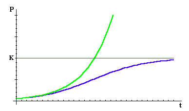
Figure: The green graph shows exponential growth while the blue graph shows logistic growth.
P.F. Verhurlst was a Belgium mathematician who studied logistic growth modeling in the 19th century. In 1840, using census data and modeling, Verhurlst predicted what the population of the United States would be in the year 1940. He was off by less than 1% (Lipkin & Smith, 2004).
Using the applet below created by melbapplets (2015), explore the logistic model for population growth. You can change the carrying capacity by dragging the green dotted line, the inital population size by dragging the red point p0, and the rate by dragging the slider.
Note the models above are derived from differential equations that are based on assumptions about the rate of change of a population. To learn more about the intuition behind the logistic differential equation, watch the video below created by Sal Khan.
Radioactive Decay
In chemistry, an isotope is a form of an element that has the same number of protons (that's what makes it the same element), but different numbers of neutrons. For example, the most common form of the element carbon is carbon-12 that has 6 protons and 6 neutrons. However, a well-known isotope of carbon is carbon-14 that has 6 protons and 8 neutrons ("Isotopes", 2018).
Some forms of elements are more stable than others. An unstable atom may undergo radioactive decay, or lose energy by emitting ionizing radiation, in order to become more stable. This decay is measured in half-lives, or the amount of time it takes for half the original isotope to decay ("Radioactive Decay", n.d.). Radioactive decay is exponential and the mass of a substance after radioactive decay can be calculated using the following formula:
m=m0e-kt
where m0 is the initial mass of the substance, k is the decay constant, and t is time (Maor, 1994).
Below is a table containing the half-lives and decay constants of various isotopes.
Isotope
Half-Life
Decay Constant
Uranium 238
4.5x10⁹ years
5.0x10⁻¹⁸
Carbon 14
5570 years
3.9x10⁻¹²
Radon 220
52 seconds
1.33x10⁻²
Lithium 8
6x10-20 seconds
1.2x10¹⁹
Using the applet below created by Relix & Are (2011), explore the radioactive decay of five different elements.
Archeologists use their knowledge of carbon-14 and its radioactive decay in a process known as carbon dating in order to calculate the age of an object ("Isotopes", 2018).